Steps 1-6

Load the R packages we will use.

library(tidyverse)
library(echarts4r)  #install this package before using
library(hrbrthemes) #install this package before using

Read the data in the files, drug_cos.csv, health_cos.csv in to R and assign to the variables drug_cos and health_cos, respectively

drug_cos  <- read_csv("https://estanny.com/static/week6/drug_cos.csv")
health_cos  <- read_csv("https://estanny.com/static/week6/health_cos.csv")

Use glimpse to get a glimpse of the data

drug_cos %>% glimpse()

Rows: 104
Columns: 9
$ ticker       <chr> "ZTS", "ZTS", "ZTS", "ZTS", "ZTS", "ZTS", "ZTS"~
$ name         <chr> "Zoetis Inc", "Zoetis Inc", "Zoetis Inc", "Zoet~
$ location     <chr> "New Jersey; U.S.A", "New Jersey; U.S.A", "New ~
$ ebitdamargin <dbl> 0.149, 0.217, 0.222, 0.238, 0.182, 0.335, 0.366~
$ grossmargin  <dbl> 0.610, 0.640, 0.634, 0.641, 0.635, 0.659, 0.666~
$ netmargin    <dbl> 0.058, 0.101, 0.111, 0.122, 0.071, 0.168, 0.163~
$ ros          <dbl> 0.101, 0.171, 0.176, 0.195, 0.140, 0.286, 0.321~
$ roe          <dbl> 0.069, 0.113, 0.612, 0.465, 0.285, 0.587, 0.488~
$ year         <dbl> 2011, 2012, 2013, 2014, 2015, 2016, 2017, 2018,~

health_cos %>% glimpse()

Rows: 464
Columns: 11
$ ticker      <chr> "ZTS", "ZTS", "ZTS", "ZTS", "ZTS", "ZTS", "ZTS",~
$ name        <chr> "Zoetis Inc", "Zoetis Inc", "Zoetis Inc", "Zoeti~
$ revenue     <dbl> 4233000000, 4336000000, 4561000000, 4785000000, ~
$ gp          <dbl> 2581000000, 2773000000, 2892000000, 3068000000, ~
$ rnd         <dbl> 427000000, 409000000, 399000000, 396000000, 3640~
$ netincome   <dbl> 245000000, 436000000, 504000000, 583000000, 3390~
$ assets      <dbl> 5711000000, 6262000000, 6558000000, 6588000000, ~
$ liabilities <dbl> 1975000000, 2221000000, 5596000000, 5251000000, ~
$ marketcap   <dbl> NA, NA, 16345223371, 21572007994, 23860348635, 2~
$ year        <dbl> 2011, 2012, 2013, 2014, 2015, 2016, 2017, 2018, ~
$ industry    <chr> "Drug Manufacturers - Specialty & Generic", "Dru~

Which variables are the same in both data sets

names_drug  <- drug_cos  %>%  names() 
names_health  <- health_cos  %>%  names() 
intersect(names_drug, names_health)

[1] "ticker" "name"   "year"

[1] “ticker” “name” “year”

Select subset of variables to work with

For drug_cos select (in this order): ticker, year, grossmargin
- Extract observations for 2018
- Assign output to drug_subset
For health_cos select (in this order): ticker, year, revenue, gp, industry
- Extract observations for 2018
- Assign output to health_subset

drug_subset  <- drug_cos  %>% 
  select(ticker, year, grossmargin)  %>% 
  filter(year == 2018)

health_subset  <- health_cos  %>%
  select(ticker, year, revenue, gp, industry)  %>% 
  filter(year == 2018)

Keep all the rows and columns drug_subset join with columns in health_subset

drug_subset  %>% left_join(health_subset)

# A tibble: 13 x 6
   ticker  year grossmargin     revenue          gp industry          
   <chr>  <dbl>       <dbl>       <dbl>       <dbl> <chr>             
 1 ZTS     2018       0.672  5825000000  3914000000 Drug Manufacturer~
 2 PRGO    2018       0.387  4731700000  1831500000 Drug Manufacturer~
 3 PFE     2018       0.79  53647000000 42399000000 Drug Manufacturer~
 4 MYL     2018       0.35  11433900000  4001600000 Drug Manufacturer~
 5 MRK     2018       0.681 42294000000 28785000000 Drug Manufacturer~
 6 LLY     2018       0.738 24555700000 18125700000 Drug Manufacturer~
 7 JNJ     2018       0.668 81581000000 54490000000 Drug Manufacturer~
 8 GILD    2018       0.781 22127000000 17274000000 Drug Manufacturer~
 9 BMY     2018       0.71  22561000000 16014000000 Drug Manufacturer~
10 BIIB    2018       0.865 13452900000 11636600000 Drug Manufacturer~
11 AMGN    2018       0.827 23747000000 19646000000 Drug Manufacturer~
12 AGN     2018       0.861 15787400000 13596000000 Drug Manufacturer~
13 ABBV    2018       0.764 32753000000 25035000000 Drug Manufacturer~

Question: join_ticker

Start with drug_cos
Extract observations for the ticker BIIB from drug_cos
Assign output to the variable drug_cos_subset

drug_cos_subset  <- drug_cos  %>% 
  filter(ticker == "BIIB")

Display drug_cos_subset

drug_cos_subset

# A tibble: 8 x 9
  ticker name  location ebitdamargin grossmargin netmargin   ros   roe
  <chr>  <chr> <chr>           <dbl>       <dbl>     <dbl> <dbl> <dbl>
1 BIIB   Biog~ Massach~        0.404       0.908     0.245 0.333 0.204
2 BIIB   Biog~ Massach~        0.402       0.901     0.25  0.335 0.211
3 BIIB   Biog~ Massach~        0.432       0.876     0.269 0.355 0.233
4 BIIB   Biog~ Massach~        0.475       0.879     0.302 0.404 0.294
5 BIIB   Biog~ Massach~        0.493       0.885     0.33  0.437 0.321
6 BIIB   Biog~ Massach~        0.491       0.871     0.323 0.431 0.322
7 BIIB   Biog~ Massach~        0.495       0.867     0.207 0.407 0.209
8 BIIB   Biog~ Massach~        0.511       0.865     0.329 0.435 0.334
# ... with 1 more variable: year <dbl>

Use left_join to combine the rows and columns of drug_cos_subset with the columns of health_cos
Assign the output to combo_df

combo_df  <- drug_cos_subset  %>% 
  left_join(health_cos)

Display combo_df

combo_df

# A tibble: 8 x 17
  ticker name  location ebitdamargin grossmargin netmargin   ros   roe
  <chr>  <chr> <chr>           <dbl>       <dbl>     <dbl> <dbl> <dbl>
1 BIIB   Biog~ Massach~        0.404       0.908     0.245 0.333 0.204
2 BIIB   Biog~ Massach~        0.402       0.901     0.25  0.335 0.211
3 BIIB   Biog~ Massach~        0.432       0.876     0.269 0.355 0.233
4 BIIB   Biog~ Massach~        0.475       0.879     0.302 0.404 0.294
5 BIIB   Biog~ Massach~        0.493       0.885     0.33  0.437 0.321
6 BIIB   Biog~ Massach~        0.491       0.871     0.323 0.431 0.322
7 BIIB   Biog~ Massach~        0.495       0.867     0.207 0.407 0.209
8 BIIB   Biog~ Massach~        0.511       0.865     0.329 0.435 0.334
# ... with 9 more variables: year <dbl>, revenue <dbl>, gp <dbl>,
#   rnd <dbl>, netincome <dbl>, assets <dbl>, liabilities <dbl>,
#   marketcap <dbl>, industry <chr>

Assign the company name to co_name

co_name  <- combo_df  %>% 
  distinct(name)  %>% 
  pull()

Assign the company location to co_location

co_location  <- combo_df  %>% 
  distinct(location)  %>% 
  pull()

Assign the industry to co_industry group

co_industry  <- combo_df  %>% 
  distinct(industry)  %>% 
  pull()

Put the r inline commands used in the blanks below. When you knit the document the results of the commands will be displayed in your text.

The company Biogen Inc is located in Massachusetts; U.S.A and is a member of the Drug Manufacturers - General industry group.

Start with combo_df
Select variables (in this order): year, grossmargin, netmargin, revenue, gp, netincome
Assign the output to combo_df_subset

combo_df_subset  <- combo_df  %>% 
  select(year, grossmargin, netmargin, 
  revenue, gp, netincome)

Display combo_df_subset

combo_df_subset

# A tibble: 8 x 6
   year grossmargin netmargin     revenue          gp  netincome
  <dbl>       <dbl>     <dbl>       <dbl>       <dbl>      <dbl>
1  2011       0.908     0.245  5048634000  4581854000 1234428000
2  2012       0.901     0.25   5516461000  4970967000 1380033000
3  2013       0.876     0.269  6932200000  6074500000 1862300000
4  2014       0.879     0.302  9703300000  8532300000 2934800000
5  2015       0.885     0.33  10763800000  9523400000 3547000000
6  2016       0.871     0.323 11448800000  9970100000 3702800000
7  2017       0.867     0.207 12273900000 10643900000 2539100000
8  2018       0.865     0.329 13452900000 11636600000 4430700000

Create the variable grossmargin_check to compare with the variable grossmargin. They should be equal.
- grossmargin_check = gp / revenue
Create the variable close_enough to check that the absolute value of the difference between grossmargin_check and grossmargin is less than 0.001

combo_df_subset  %>% 
  mutate(grossmargin_check = gp / revenue,
  close_enough = abs(grossmargin_check - grossmargin) < 0.001)

# A tibble: 8 x 8
   year grossmargin netmargin     revenue          gp  netincome
  <dbl>       <dbl>     <dbl>       <dbl>       <dbl>      <dbl>
1  2011       0.908     0.245  5048634000  4581854000 1234428000
2  2012       0.901     0.25   5516461000  4970967000 1380033000
3  2013       0.876     0.269  6932200000  6074500000 1862300000
4  2014       0.879     0.302  9703300000  8532300000 2934800000
5  2015       0.885     0.33  10763800000  9523400000 3547000000
6  2016       0.871     0.323 11448800000  9970100000 3702800000
7  2017       0.867     0.207 12273900000 10643900000 2539100000
8  2018       0.865     0.329 13452900000 11636600000 4430700000
# ... with 2 more variables: grossmargin_check <dbl>,
#   close_enough <lgl>

Create the variable netmargin_check to compare with the variable netmargin. They should be equal.
Create the variable close_enough to check that the absolute value of the difference between netmargin_check and netmargin is less than 0.001

combo_df_subset  %>% 
  mutate(netmargin_check = netincome / revenue,
  close_enough = abs(netmargin_check - netmargin) < 0.001)

# A tibble: 8 x 8
   year grossmargin netmargin     revenue          gp  netincome
  <dbl>       <dbl>     <dbl>       <dbl>       <dbl>      <dbl>
1  2011       0.908     0.245  5048634000  4581854000 1234428000
2  2012       0.901     0.25   5516461000  4970967000 1380033000
3  2013       0.876     0.269  6932200000  6074500000 1862300000
4  2014       0.879     0.302  9703300000  8532300000 2934800000
5  2015       0.885     0.33  10763800000  9523400000 3547000000
6  2016       0.871     0.323 11448800000  9970100000 3702800000
7  2017       0.867     0.207 12273900000 10643900000 2539100000
8  2018       0.865     0.329 13452900000 11636600000 4430700000
# ... with 2 more variables: netmargin_check <dbl>,
#   close_enough <lgl>

Question: summarize_industry

Fill in the blanks
Put the command you use in the Rchunks in the Rmd file for this quiz
Use the health_cos data
For each industry calculate
- mean_netmargin_percent = mean(netincome / revenue) * 100
- median_netmargin_percent = median(netincome / revenue) * 100
- min_netmargin_percent = min(netincome / revenue) * 100
- max_netmargin_percent = max(netincome / revenue) * 100

health_cos  %>% 
  group_by(industry)  %>% 
  summarize(mean_netmargin_percent = mean(netincome / revenue) * 100,
            median_netmargin_percent = median(netincome / revenue) * 100,
            min_netmargin_percent = min(netincome / revenue) * 100,
            max_netmargin_percent = max(netincome / revenue) * 100
  )

# A tibble: 9 x 5
  industry          mean_netmargin_~ median_netmargi~ min_netmargin_p~
  <chr>                        <dbl>            <dbl>            <dbl>
1 Biotechnology                -4.66             7.62         -197.   
2 Diagnostics & Re~            13.1             12.3             0.399
3 Drug Manufacture~            19.4             19.5           -34.9  
4 Drug Manufacture~             5.88             9.01          -76.0  
5 Healthcare Plans              3.28             3.37           -0.305
6 Medical Care Fac~             6.10             6.46            1.40 
7 Medical Devices              12.4             14.3           -56.1  
8 Medical Distribu~             1.70             1.03           -0.102
9 Medical Instrume~            12.3             14.0           -47.1  
# ... with 1 more variable: max_netmargin_percent <dbl>

mean_netmargin_percen for the industry Medical Care Facilities is 6.10%
median_netmargin_percent for the industry Medical Care Facilities is 6.46%
min_netmargin_percent for the industry Medical Care Facilities is 1.40%
max_netmargin_percent for the industry Medical Care Facilities is 8.30%

Question: inline_ticker

Fill in the blanks
Use the health_cos data
Extract observations for the ticker ILMN from health_cos and assign to the variable health_cos_subset

health_cos_subset  <- health_cos  %>% 
  filter(ticker == "ILMN")

Display health_cos_subset

health_cos_subset

# A tibble: 8 x 11
  ticker name       revenue     gp    rnd netincome assets liabilities
  <chr>  <chr>        <dbl>  <dbl>  <dbl>     <dbl>  <dbl>       <dbl>
1 ILMN   Illumina ~  1.06e9 7.09e8 1.97e8  86628000 2.20e9  1120625000
2 ILMN   Illumina ~  1.15e9 7.74e8 2.31e8 151254000 2.57e9  1247504000
3 ILMN   Illumina ~  1.42e9 9.12e8 2.77e8 125308000 3.02e9  1485804000
4 ILMN   Illumina ~  1.86e9 1.30e9 3.88e8 353351000 3.34e9  1876842000
5 ILMN   Illumina ~  2.22e9 1.55e9 4.01e8 462000000 3.69e9  1839194000
6 ILMN   Illumina ~  2.40e9 1.67e9 5.04e8 454000000 4.28e9  2011000000
7 ILMN   Illumina ~  2.75e9 1.83e9 5.46e8 725000000 5.26e9  2508000000
8 ILMN   Illumina ~  3.33e9 2.3 e9 6.23e8 826000000 6.96e9  3114000000
# ... with 3 more variables: marketcap <dbl>, year <dbl>,
#   industry <chr>

In the console, type ?distinct. Go to the help pane to see what distinct does
In the console, type ?pull. Go to the help pane to see what pull does

Run the code below

health_cos_subset  %>% 
  distinct(name) %>%  
  pull(name)

[1] "Illumina Inc"

Assign the output to co_name

co_name  <- health_cos_subset  %>% 
  distinct(name) %>% 
  pull(name)

You can take output from your code and include it in your text.

The name of the company with ticker ILMN is Illumina Inc

In following chuck

Assign the company’s industry group to the variable co_industry

co_industry  <- health_cos_subset  %>% 
  distinct(industry) %>% 
  pull()

This is outside the R chunk. Put the r inline commands used in the blanks below. When you knit the document the results of the commands will be displayed in your text.

The company Illumina Inc is a member of the Diagnostics & Research group.

Steps 7-11

Prepare the data for the plots

start with health_cos THEN
group_by industry THEN
calculate the median research and development expenditure as a percent of revenue by industry
assign the output to df

df <- health_cos  %>% 
  group_by(industry)  %>%
  summarize(med_rnd_rev = median(rnd/revenue))

Use glimpse to glimpse the data for the plots

df  %>% glimpse()

Rows: 9
Columns: 2
$ industry    <chr> "Biotechnology", "Diagnostics & Research", "Drug~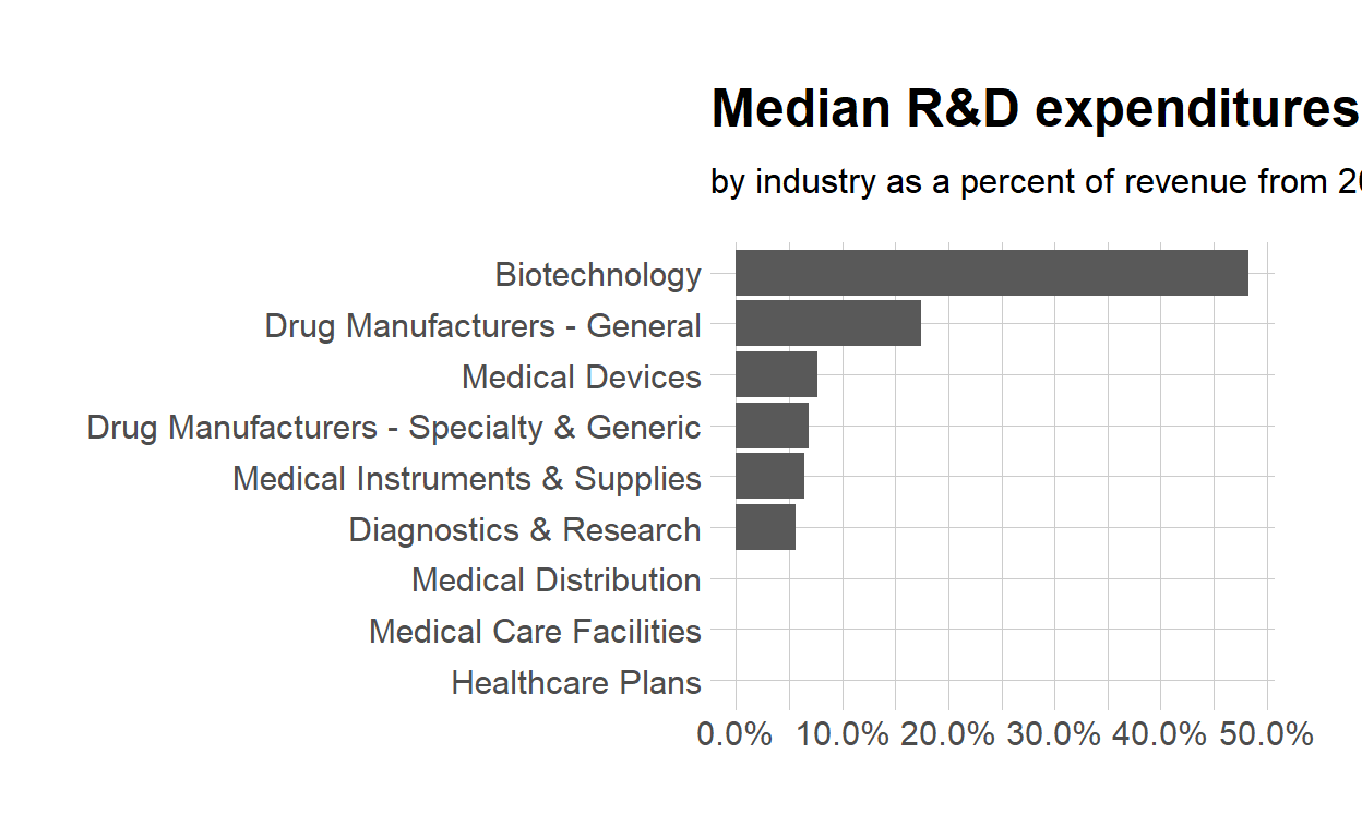
$ med_rnd_rev <dbl> 0.48317287, 0.05620271, 0.17451442, 0.06851879, ~

Create a static bar chart

use ggplot to initialize the chart
data is df
the variable industry is mapped to the x-axis
- reorder it based the value of med_rnd_rev
the variable med_rnd_rev is mapped to the y-axis
add a bar chart using geom_col
use scale_y_continuous to label the y-axis with percent
use coord_flip() to flip the coordinates
use labs to add title, subtitle and remove x and y-axes
use theme_ipsum() from the hrbrthemes package to improve the theme

ggplot(data = df, 
       mapping = aes(
         x = reorder(industry, med_rnd_rev ),
         y = med_rnd_rev
         )) +
  geom_col() + 
  scale_y_continuous(labels = scales::percent) +
  coord_flip() +
  labs(
    title = "Median R&D expenditures",
    subtitle = "by industry as a percent of revenue from 2011 to 2018",
    x = NULL, y = NULL) +
  theme_ipsum()

Save the previous plot to preview.png and add to the yaml chunk at the top

ggsave(filename = "preview.png", 
       path = here::here("_posts", "2022-02-09-joining-data"))

Create an interactive bar chart using the package echarts4r

start with the data df
use arrange to reorder med_rnd_rev
use e_charts to initialize a chart
- the variable industry is mapped to the x-axis
add a bar chart using e_bar with the values of med_rnd_rev
use e_flip_coords() to flip the coordinates
use e_title to add the title and the subtitle
use e_legend to remove the legends
use e_x_axis to change format of labels on x-axis to percent
use e_y_axis to remove labels on y-axis-
use e_theme to change the theme. Find more themes here

df  %>% 
  arrange(med_rnd_rev)  %>%
  e_charts(
    x = industry
    )  %>% 
  e_bar(
    serie = med_rnd_rev, 
    name = "median"
    )  %>%
  e_flip_coords()  %>% 
  e_tooltip()  %>% 
  e_title(
    text = "Median industry R&D expenditures", 
    subtext = "by industry as a percent of revenue from 2011 to 2018",
    left = "center") %>% 
  e_legend(FALSE) %>% 
  e_x_axis(
    formatter = e_axis_formatter("percent", digits = 0)
    )  %>%
  e_y_axis(
    show = FALSE
  )  %>% 
  e_theme("infographic")

Joining Data

Steps 1-6

Question: join_ticker

Question: summarize_industry

Question: inline_ticker

Steps 7-11